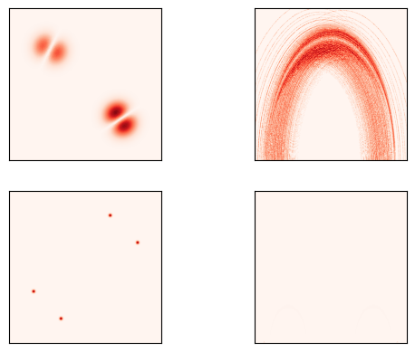
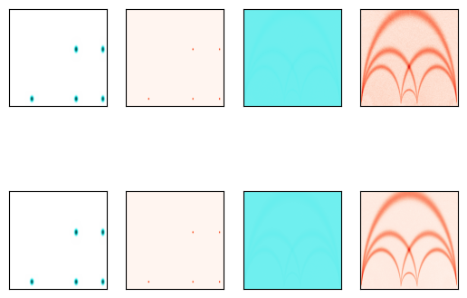
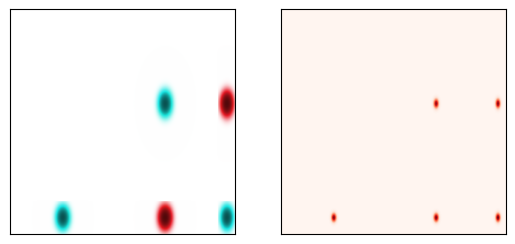
# calculate Ruelle distribution beyond delta-1 for conventional torus params
HIGHER_RESONANCE: Final[complex] = -0.8847
systemType = MapSystemType.FUNNEL_TORUS
systemInitArgs = {"outerLen": 10.0, "innerLen": 10.0, "angle": np.pi / 2.00}
N_MAX = 7

poincareArgs = {
    "sigma": 1e-3,
    "refinementLevel": 0,
    "minusIndices": [1, 2, 3],
    "plusIndices": [0, 1],
}
fundamentalDomainArgs = {
    "sigma": 6e-2,
    "refinementLevel": 0,
}

_, (axs1, axs2) = plt.subplots(2, 4)

for i, axs in enumerate((axs1, axs2)):
    for j, (integralType, args) in enumerate(
        zip(
            [OrbitIntegralType.POINCARE, OrbitIntegralType.FUNDAMENTAL_DOMAIN],
            [poincareArgs, fundamentalDomainArgs],
        )
    ):
        ruelle = RuelleDistribution(
            systemType,
            systemInitArgs=systemInitArgs,
            integralType=integralType,
            numSupportPts=300,
            **args,
        )

        higherDistribution = ruelle(
            np.array([HIGHER_RESONANCE], dtype=np.complex128), nMax=N_MAX + i
        )[0]

        # create a phase-lightness representation of the distribution
        absoluteValue = np.abs(higherDistribution)
        argument = np.angle(higherDistribution)
        hue = (argument + np.pi) / (2 * np.pi) + 0.5
        lightness = 1.0 - 1.0 / (1.0 + absoluteValue**0.2)
        saturation = 0.8

        rgb = np.array(np.vectorize(hls_to_rgb)(hue, lightness, saturation))
        rgb = rgb.swapaxes(0, 2).swapaxes(0, 1)

        axs[2 * j].imshow(np.abs(1.0 - rgb), cmap="Reds", origin="lower")
        axs[2 * j].set_xticks([])
        axs[2 * j].set_yticks([])

        axs[2 * j + 1].imshow(
            np.abs(higherDistribution), cmap="Reds", origin="lower"
        )
        axs[2 * j + 1].set_xticks([])
        axs[2 * j + 1].set_yticks([])

plt.show()